AI Ethnicity Detector vs DNA Test: Counting the Evidence Channels
One tool returns a label and the other returns a vector with an interval. The gap is not accuracy but how many independent channels each one can read.
One returns a label, one returns a vector
A photo-based ethnicity detector is a classifier. It is trained on a fixed label set, and its output is a distribution over that set which must sum to one. That constraint sounds technical and is not: the architecture has no slot for none of these, so a face belonging to no label in the training set still receives its best-fitting label, usually with a confidence figure attached. A DNA test is an estimator. It returns proportions that sum to one hundred percent, each carrying an interval, and the interval is where much of the useful information sits. A report that says 42 percent with a range of 38 to 46 is a different kind of claim from a score of 0.42, even though both are numbers between zero and one.
The 85 percent is a per-locus figure
Lewontin's 1972 apportionment found that about 85.4 percent of human genetic variation sits within populations rather than between them, and that figure is still quoted correctly. Richard Edwards pointed out in 2003 that the number is computed locus by locus, and that information from many loci accumulates when they are considered together. Rosenberg and colleagues demonstrated the arithmetic in 2002 with 377 microsatellites, recovering five clusters from a worldwide sample. Both statements hold at the same time, because one describes a single marker's diagnostic power and the other describes what happens when you have hundreds of them.
What makes ancestry recoverable from DNA is therefore not that any one marker decides anything. It is the count of independent markers, and the fact that they are inherited in blocks, so that neighbouring sites carry correlated information. Panels are built around that property: a few hundred ancestry-informative markers, selected for large frequency differences between reference groups, will separate those groups far better than any single marker in the set can. Remove the count and the recoverability goes with it.
How many channels does a face carry
Pigmentation is the exception where a few loci carry large effects: SLC24A5 and SLC45A2 for skin, HERC2 and OCA2 for eye colour, MC1R and TYR in the same pathway. Craniofacial shape is the opposite case. It is highly polygenic, the effect of any single locus is small, and a large share of the measured variance tracks age, sex, and body mass rather than ancestry. Layered on top are the variables a photograph adds and a genotype does not: focal length, light direction, pose, expression, and compression. The face is a low-dimensional, high-noise channel, and a detector's ceiling is set by the channel before any model is chosen.
The Inuid entry in this catalogue is a good illustration of what the channel can and cannot support. It records a trait list for Arctic coastal populations, down to the smallest nasal opening described anywhere, and cites Neumann 1952 and Levin 1963. That is a statement about a documented sample in a region, assembled from measurements taken decades ago. It is not a claim about the nose of any person who walks past a camera today, and no classifier trained on photographs can recover the difference.
Where the DNA test's own floor sits
A centimorgan is defined as a one percent chance of a crossover in a single generation. A segment seven centimorgans long therefore survives one generation with probability of roughly 0.93, and its expected lifetime is about 14 generations, which at 28 years per generation is close to 390 years. Segments below the threshold a laboratory uses are usually not reported, and the small-percentage trace categories in consumer reports are exactly where that floor applies. This matters for the comparison because the floor lands in the same centuries as the baseline this catalogue uses, roughly 1500 years ago. Both instruments go quiet at a similar depth, for entirely different reasons.
The DNA side still has three structural advantages, and they are worth stating plainly. It gives an interval instead of a point. It publishes the reference panel its estimates are computed against. And the raw data file is portable, so a second laboratory can re-analyse the same genotypes without asking for another sample. For anyone who wants to check a claim rather than accept it, that combination is the stronger offer of the two, and it is the reason a report can be argued with while a bare confidence score usually cannot.
What each one is scored against
Neither tool is scored against ancestry itself. 1000 Genomes Phase 3 released 2,504 samples from 26 populations, and the Human Genome Diversity Project panel covers around 51 populations with roughly a thousand individuals. Both were assembled from volunteers whose labels came from geography and self-description. A detector is scored the same way, against a caption, a self-report, or a photographer's note attached to an image. Two different instruments, one shared weakness: the ground truth is administrative, and it inherits the assumption that a person has one origin and that the origin has a name.
The map both of them assume
Both tools assume a stable map, and the map has not been stable. The photographs used to train detectors are mostly recent, but the populations they represent have been moving for centuries: Atlantic trade, nineteenth-century labour migration, the displacements after 1945, and the urbanisation that followed. A model fitted to that mixture will be most confident where the mixture is thinnest and least reliable exactly where people have moved most. A reference panel built from volunteers with four grandparents from one region carries the same blind spot, since it selects for the people whose families stayed put. The catalogue entries here are open about their own version of this problem: they describe samples collected between roughly 1880 and 1960, against a stated baseline of about 1500 years ago.
Which reader each one suits
If the question is what the literature recorded about appearance in a region, a catalogue entry answers it and shows its work. Gobid was named Central Asiatic by Yarkho in 1929, renamed by later authors, and defined by a brachycephalic vault and a strong epicanthus across the Gobi and southern Siberia; Danakil was described for the Afar and neighbouring groups in a depression averaging above 34 degrees Celsius, and the entry notes it as the shortest of the Ethiopid forms. You can check those claims against Yarkho, Eickstedt, or Biasutti and disagree with them on the evidence. If the question is how much of a genome matches a named reference population, only a DNA test answers it, and only with the interval attached. A photo detector answers a third question: which of its labels does this picture most resemble. That is a reasonable thing to want from a game or a demonstration, and it is fast, needs no sample, and costs nothing on most free tiers.
The practical split follows from that. For a documented appearance pattern with a distribution and a citation, read the catalogue. For a proportion with an error bar, take the test and keep the raw file. For a quick label on a photograph, use a detector and read its number as a similarity, not as a finding. None of the three is a worse answer than the others; each answers a narrower question than the one it is usually asked.
Frequently Asked Questions
- Can an AI ethnicity detector replace a DNA test?
- No, because the two do not measure the same thing. A detector reads surface appearance from a photograph and returns one label from a fixed set, with no way to answer none of these. A DNA test reads inherited markers and returns proportions with intervals against a published reference panel. Appearance and ancestry are related but not interchangeable: pigmentation loci have large effects and are easy to see, while most of the genome's ancestry signal is invisible in a face. One can be a fast guess and the other a measurement, but neither substitutes for the other.
- Why do DNA tests disagree with each other about the same person?
- Mostly because they use different reference panels and different minimum segment lengths. A proportion is computed relative to whichever populations the laboratory chose to include, so a report with 40 reference groups will carve the same genome differently from one with 26. Minimum segment thresholds also differ, and segments below the threshold are dropped rather than reported as uncertain. The genotypes can be identical while the percentages differ, which is why the raw data file is worth keeping: it lets a second laboratory recompute the estimate.
- How far back can either method actually see?
- For DNA, the practical limit comes from recombination. A segment shrinks by roughly half every generation in expectation, so a seven centimorgan block has an expected lifetime near 14 generations, or about four centuries, before it is likely to be broken. Shorter blocks are usually filtered out. For a photograph, the limit is different in kind: it records a living face, and it says nothing about inheritance at all. Neither method reaches the roughly 1500-year baseline that a historical catalogue of documented appearance patterns is describing.
Related Phenotypes
Faces from the encyclopedia that appear in this article. Open any entry for its full description, distribution, and references.
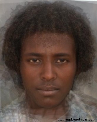
Danakil
East Africa
Specialised Ethiopid type living in the hottest region of the world: the Danakil depression of Eritrea and Northern Ethiopia, with an annual...
Gobid
Central Asia
Tungid variety of the vast Central Asian deserts and steppes, e.g. the Gobi and Southern Siberia. Developed in ancient stock-farming nomads ...
Inuid
Arctic
Eskimid proper type, ranging over the vast, sparsely populated tundra along the icy coasts of Alaska, Nunavut, and Labrador (Canada) to Gree...
Test what you learned
Put your eye for regional faces to work in the daily quiz — a composite face, a world map, and your best guess.